The post contains my writeup to IMGPROJ - Image Projections SPOJ problem.

1. Prerequisites

It is assumed that the reader is familiar with segment trees. This article contains a thorough description of segment trees.

1. Problem description

Full problem statement is provided here.

In short, we are given a definition of diagonal projection:
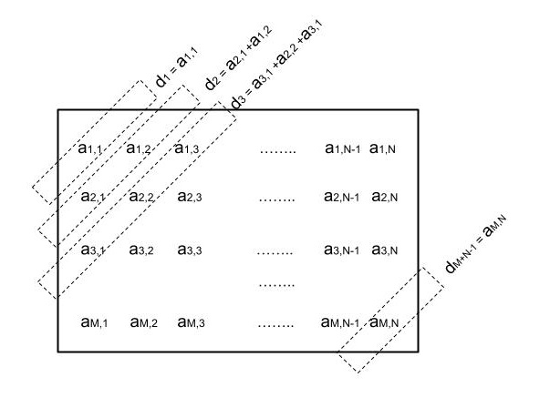
Diagonal projection of a matrix \(I\) with \(M\) rows and \(N\) columns is the vector \((d_1, ... , d_{M + N - 1})\) where \(d_i = \sum_{x+y-1=i}\) I[x][y].
On the program input there is a matrix. Our task is to compute its diagonal projection.
An important note: Rows of the matrix are provided in run length encoding. Also, the returned diagonal projection has to be run-length encoded.
Through the rest of the article I will refer to i’th “{intensity-count} {intensity-value} “ pair in the j’th row in run-length encoded input matrix as \(\textit I_{RLE}[i][j]\). \(\textit I_{RLE}[i][j].value\) will denote intensity value and \(\textit I_{RLE}[i][j].count\) will denote size of \(\textit I_{RLE}[i][j]\).

Visualization of diagonal projection:

Width of each image is at most \(10^9\) and height is at most \(10^3\). Total size of the input does not exceed 4 MB.

2. Initial attempts

It is easy to spot, that \(\textit I_{RLE}[i][j]\) will add \(\textit I_{RLE}[i][j].value\) to range of elements \(d_{i + p}, d_{i+p+1}, ... , d_{i+p+count-1}\) where \(p\) is equal to \(\sum_{k < i}I_{RLE}[i][j].count\) and \(count\) is \(\textit I_{RLE}[i][j].count\).

My initial idea was to create a vector of length \(M+N-1\) to hold diagonal projection. Then for each \(\textit I_{RLE}[i][j]\) add \(\textit I_{RLE}[i][j].value\) to \(\textit I_{RLE}[i][j].count\) elements of the diagonal projection the pair concerns.

A simplified algorithm for computing diagonal projection looked like this:

Unfortunately my submit was getting time limit exceeded status.

Complexity of this algorithm is equal to the size of matrix (\(M \times N\)), because each matrix cell is processed exactly once in constant time in one RLE pair. Maximum matrix width is \(10^9\) and maximum height is \(10^3\), so the algorithm may need number of computations of order \(10^9 \cdot 10^3=10^{12}\). I needed a faster solution.

3. Improved solution

The task statement guarantees that the input size is at most 4 MB. Each \(\textit I_{RLE}[i][j]\) occupies at least 4 bytes of input (1 byte for count part, 1 byte for value part and 2 bytes for spaces). Therefore there are no more than \(4 \cdot 10^6 / 4 = 10^6\) pairs.

Lets divide the vector \((d_1, d_2, ..., d_{M+N-1})\) into chunks where each chunk \(c = (d_{n}, d_{n+1}, ... , d_{n+m})\) is the biggest subvector such that there is no \(\textit I_{RLE}[i][j]\) that adds values to some, but not all elements of \(c\). In other words, lets take starting points (first elements to which a value will be added) of all \(\textit I_{RLE}[i][j]\) within diagonal projection and split projection in these points.

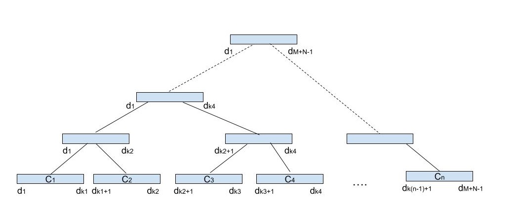
I came up with an idea to solve the problem using a segment tree. Each leaf holds one of the forementioned chunks. Each node (including leaves) contains a sum that should be added to \(d_i\)’s from chunks in its subtree. Number of leaves will be the minimum power of two greater than the number of chunks. Size of the whole tree will be twice as big as the number of its leaves (binary tree property).
Every node will hold the following elements:

• left-most index of diagonal projection part in chunks of its subtree
• right-most index of diagonal projection part in chunks of its subtree
• value that should be added to all diagonal projection elements in the range determined by left-most and right-most diagonal projection indexes.

Diagram of the segment tree is shown below:

Each \(\textit I_{RLE}[i][j]\) will add a value to diagonal projection elements in one or more consecutive chunks. Therefore values coming from these pairs can be added into the tree as intervals using standard segment tree insertion procedure.
After inserting all \(\textit I_{RLE}[i][j]\), final values of diagonal projection elements in a given chunk can be determined by summing values in the path from root to the leaf with the chunk.

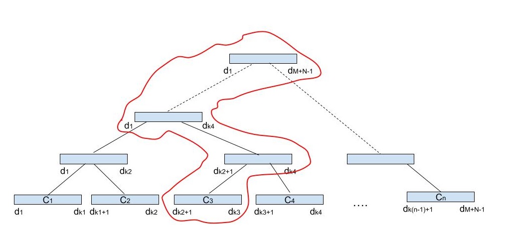
For example to compute diagonal projection between \(d_{k_2+1}\) and \(d_{k_3}\) from the previous diagram values from nodes in the path from \(c_3\) to the tree root must be summed:

After computing diagonal projection values for all chunks we need to return them in run-length encoding. Obviously, computing diagonal projection elements within one chunk will have the same value. We cannot however directly convert each chunk into rle-pair and return it as a problem solution. It may happen that neighboring chunks will have the same diagonal projection values. RLE pairs should be as long as possible, so consecutive neighboring chunks with the same diagonal projection values need to be merged into one RLE-pair. After creating list of RLE-pairs from chunks and merging consecutive pairs with the same value, the rle-pair list can be returned as a problem solution.

Putting this all together we can compute running length encoded diagonal projection with the following algorithm:

1. Compute start and end indexes of all \(\textit I_{RLE}[i][j]\) within diagonal projection to get chunk boundaries.
2. Create a segment tree whose leaves hold a range from chunks. Each node in the tree holds a value that must be added to all projection elements within in the range defined by its subtree.
3. Insert every \(\textit I_{RLE}[i][j]\) into the tree using standard segment tree insertion procedure.
4. Compute final diagonal projection values in every chunk by summing values from root node to the chunk leaf.
5. Convert each chunk into RLE-pair, merge consecutive pairs with the same values and return the RLE-list.

The above solution was accepted by SPOJ judge.

3.1 Algorithm complexity

Lets summarize time complexities of individual algorithm steps:

1. Computing start and end indexes of \(\textit I_{RLE}[i][j]\) may take \(O(N \cdot M)\). Previous analysis shows that number of pairs is at most \(10^6\) and each pair may be processed in constant time.
2. Size of a segment tree with chunks is twice the number of leaves (aligned to a power of two). Time complexity of creating and filling with chunk range information is proportional to the size of the tree, which is \(O(N + M)\). Number of chunks is at most \(10^6\) so tree size is at most \(2 \cdot 2 \cdot 10^6\) (multiplied by 4 to incorporate whole tree size and align tree to the power of 2).
3. Inserting a single element to a segment tree has time complexity \(O( log(\) tree size \())\). There are \(O(N \cdot M)\) \(\textit I_{RLE}[i][j]\) pairs and tree size is \(O(N + M)\). So upper time bound for inserting all elements into the tree is \(O(N \cdot M \cdot log (N + M))\). Tree size is at most \(2 \cdot 2 \cdot 10^6\) and number of RLE-pairs is at most \(10^6\) so number of all operations (a single operation is a constant-time processing in a tree node) is no more than \(1.6 \cdot 10^6\).
4. Computing diagonal projection values for a single chunk in the segment tree has time complexity \(O( log(\) tree size \())\). There are \(O(N + M)\) chunks and tree size is \(O(N + M)\). So upper time bound for computing projection for all chunks in the tree is \(O((N + M) \cdot log (N + M))\). Taking into account tree size and chunks count, there are will be at most \(1.6 \cdot 10^6\) operations.

Overall algorithm complexity is \(O(N \cdot M \cdot log (N + M))\) which is bigger than the initial solution. However, because of the additional constraints on the number of \(\textit I_{RLE}[i][j]\), the number of computations is of order \(10^6\) which is less than in the previous approach.

4. Implementation

I implemented the solution to this problem in Rust. The code is available here.